We spent a month (during May/June 2026) optimizing Qwen-3.5-397B-A17B-FP8 inference using Ironwood TPUs. Our challenge was to investigate whether closing the gap with NVIDIA B200 GPUs was possible for this relatively new model architecture.

We were interested in the following performance optimizations:

• maximizing throughput/TPU with a 10 tok/s/user interactivity floor,

• maximizing throughput/TPU with a 115 tok/s/user interactivity floor,

• maximizing tok/s/user at any concurrency

Importantly, we were not investigating speculative decoding or multi-token prediction . Neither were we performing any post-training methods that could impact quality or accuracy. We were primarily focused on speeding up the raw autoregressive token performance.

In a single month, without prior experience with the TPU ecosystem, we significantly improved performance by up to 5x compared to the stock vllm-tpu fork, approaching B200 performance on the high-throughput regime, and outperforming B200 on the high interactivity regime! This confirms that software is a real gap when it comes to performance engineering, and that Makora's automation tools are portable across hardware.

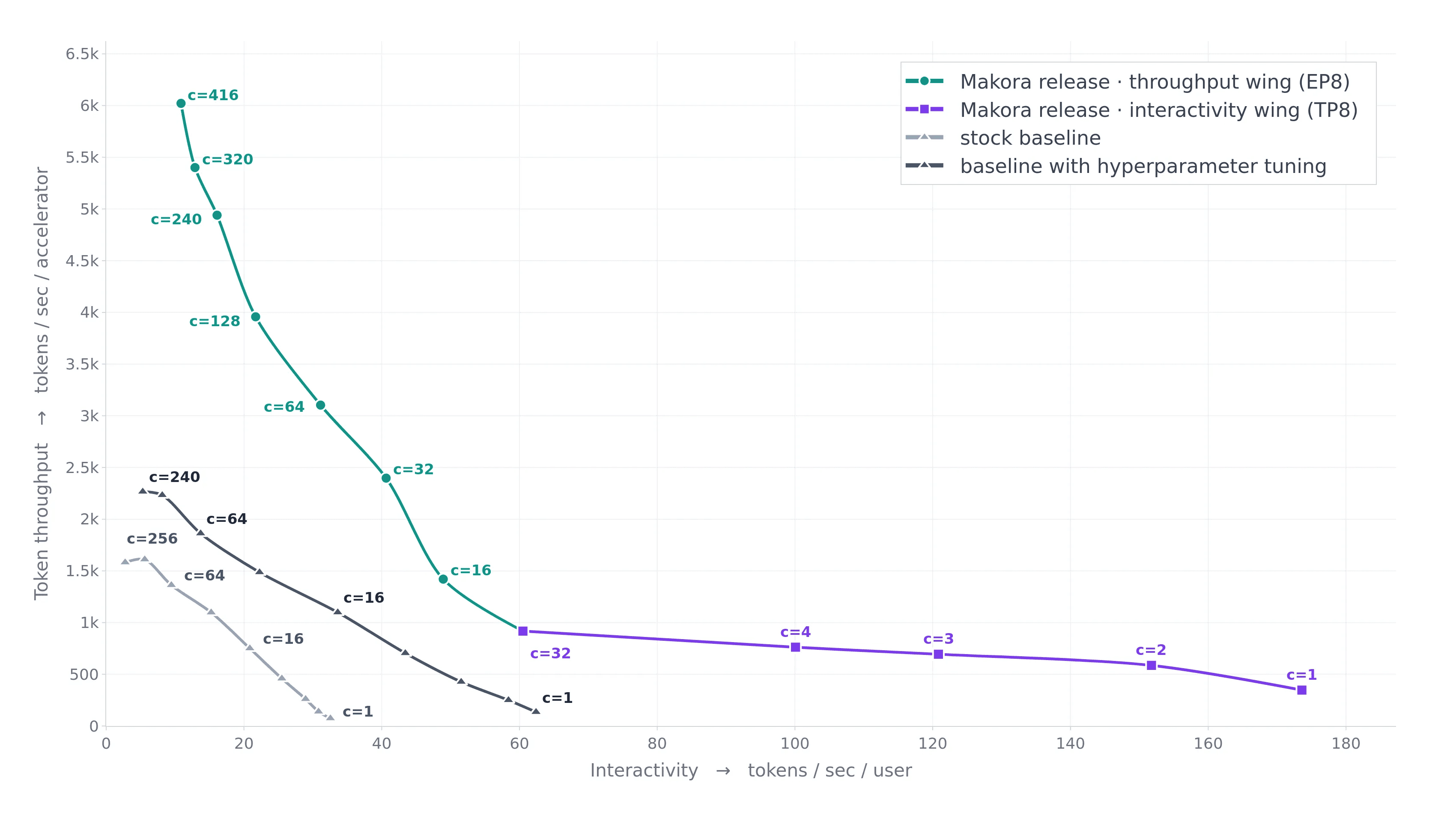
Higher is more total throughput, more to the right is more tok/s/user, c is the number of concurrent requests.

In other words:

• light grey is what you get if you run vllm serve 🐌

• dark grey is what you get if your performance engineer tunes vLLM hyperparameters for you 🐌🏁

• green and purple curves are what you get with Makora 🦈

At the time this post was written, the optimization changes were in the process of being upstreamed to the vLLM core and vLLM TPU backend repositories. Below we will describe the high interactivity optimizations we came up with, then we will outline some of performance automation tools used to achieve our results.

Interactivity is a strange beast...

Until recently, LLM inference was focused on throughput — it was assumed extreme concurrency is all you need, and serving LLMs is only cost-effective at a massive scale. The rise of coding agents changed that dynamic, as reaching 50, 100 or 150 tok/s/user became very valuable for interactive, synchronous work with a human operator.

As LLMs such as Qwen are autoregressive, the number of concurrent requests puts a hard cap on possible parallelism. You cannot reliably generate the n+1-th token without first running the n-th token through the entire model. As such, maximizing low-concurrency interactivity becomes a game of hiding as much memory access latency as possible. Bandwidth and compute capacity are fully utilized only for a fraction of a step's runtime, and the rest of the time is spent starved for data to process.

Qwen-3.5-397B-A17B is a massive model and, due to memory constraints, it must be deployed on 4 TPUs / 8 chiplets. 8-way tensor parallel sharding slices the weights and intermediate buffers into even smaller parts and introduces further waits on collective operations.

...and so are TPUs

GPU kernels are designed around hundreds of compute units, each processing several warps (Nvidia) or wavefronts (AMD) at the same time, with multiple level of schedulers arbitrating which instructions should run at any given time. A block of warps may share a tiny, kilobytes-sized memory buffer called shared memory as a scratchpad. A single GPU kernel runs in thousands of parallel, resource-constrained invocations, with each warp delivering a small slice of the result. Even decades later, the legacy of the first programmable shader processors is visible in GPU design.

A Google TPU doesn't do any of that. Instead, in just a few cycles, a Tensor Core VPU processes up to 128x8 elements each instruction, growing up to 256x256 for MXU operations, with an efficient memory loading pipeline keeping the arithmetic units fed. Where a GPU runs thousands of tiny parallel programs, a TPU has one kernel invocation running at a time, with no interruptions.

GPUs have multiple levels of cache — L2, L1, sometimes L0. TPU designers dropped the concept of device-managed caches entirely — instead, they provided a huge fast-access bank called VMEM. In the Ironwood architecture, each of the two chiplets has 64MB of VMEM that the programmer can manually utilize for caching, scratch space or intermediate result storage.

If you've ever written a GPU kernel, by this point you should get excited — what can we do with all this space and processing power? How many algorithms become straightforward if you don't have to divide work into tiny slices to fit a GPU warp? Let's find out.

Grouped GEMM is overrated

Mixture of Experts inference is a well-trodden problem and preexisting, high-performance grouped GEMM implementations should, in general, be faster than bespoke custom kernels.

When decoding one request, or even 3-4 requests at a time, this is completely wrong.

Grouped GEMM relies on a straightforward observation. If we have many experts and many tokens, we should rearrange the post-attention latents so that each expert's incoming tokens are contiguous in memory. Thus, we can launch many instances of the same kernel, targeting different experts and process each expert's work in parallel.

Now, for a specific example, Qwen-3.5 uses one shared expert and ten routed experts, picked by a routing network for each token out of a set of 512.

So now imagine you have a single request to handle, a single token to decode, and a TPU. Each group has, by definition, a size of one as experts cannot be chosen twice. The input is shared for the up projection, and yet in a grouped GEMM kernel it would be duplicated ten times. Moreover, a grouped GEMM kernel is still a GEMM kernel, so it will tile in squares or rectangles for weight reuse... which doesn't happen at all, as in this scenario each expert call is a GEMV and no weight is used twice!

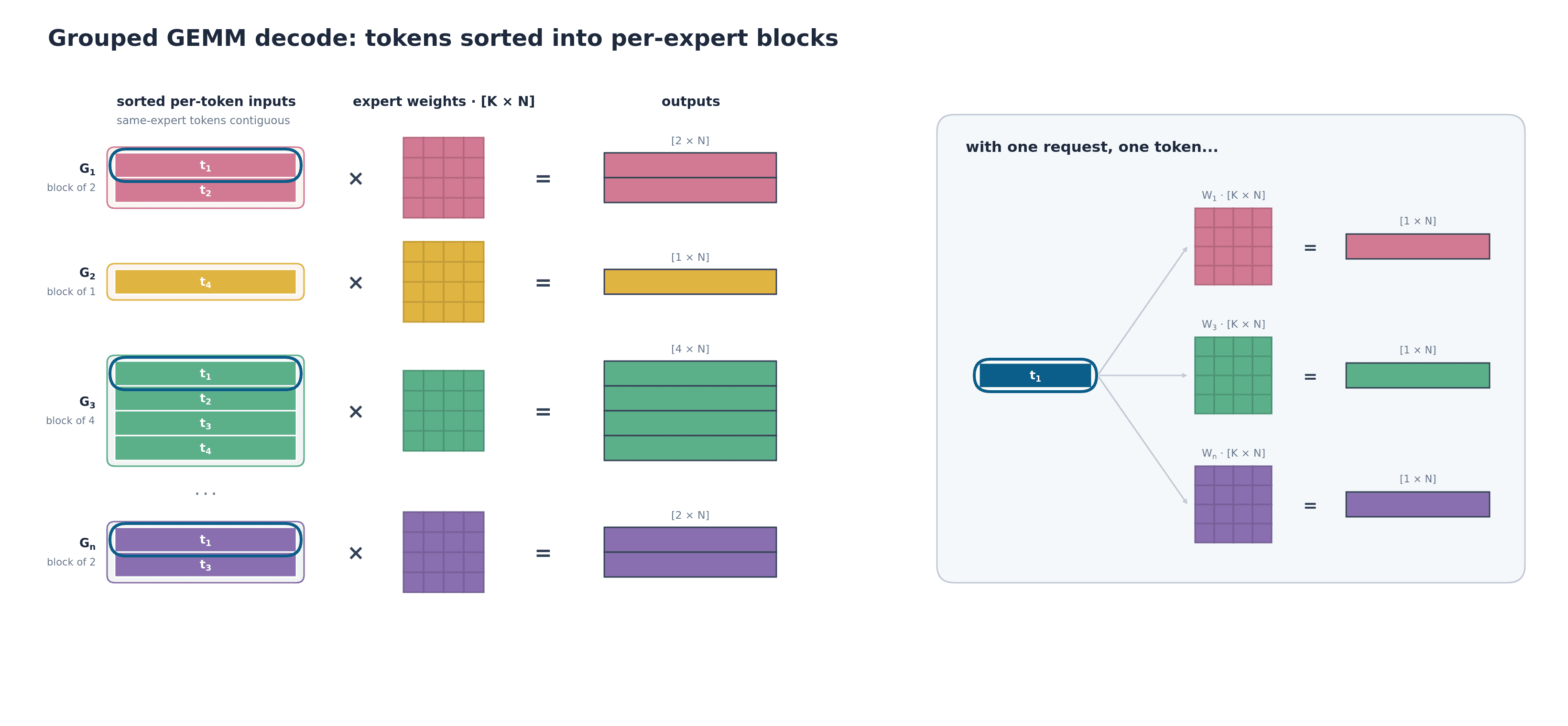
You'd think this gets better with a few requests in flight, but we measured the overlap between experts chosen with three concurrent requests — only 5% of the chosen experts were duplicated! As such, at low concurrency grouped GEMM doesn't justify its overhead.

GEMV is all you need

So let's write a custom Pallas kernel that will work with these constraints. If you've ever worked with Triton, you should find Pallas easy to read.

A seasoned performance engineer will notice this problem boils down to rotating through the expert weights as fast as possible, and everything else will be hidden in the load latency. In GPU programming, we'd reach for a lot of warps and in-warp double buffering.

On an Ironwood TPU, fortunately, we have a lot of VMEM to spare, and for a few experts at a time, we can cram a full 1/8th TP shard of each into VMEM at once. But we need to make up for just having one mega-warp. So how many experts can we load in parallel, into our VMEM "ring buffer"?

# Prime the ring: fire NBUF_ whole-expert weight DMAs up front, so up to
# NBUF_ expert loads are in flight across the HBM engines at once.
for j in range(min(NBUF_, TOP_K_)):
    pltpu.make_async_copy(rhs_ref.at[pl.ds(ids_ref[j], 1)],
                          w_bufs_ref.at[pl.ds(j, 1)],
                          sem_ref.at[j]).start()
    # ... (+ start the matching weight-scale DMA) ...

for i in range(TOP_K_):
    buf = i % NBUF_
    pltpu.make_async_copy(rhs_ref.at[pl.ds(ids_ref[i], 1)],
                          w_bufs_ref.at[pl.ds(buf, 1)],
                          sem_ref.at[buf]).wait()
    # ... (wait on the matching weight-scale DMA) ...
    w_fp8 = w_bufs_ref[buf]
    s = s_bufs_ref[buf]
    w_dequant = (w_fp8.astype(jnp.float32).reshape(K_BLOCKS, QB, N) * s) \
        .reshape(K, N).astype(DTYPE_LHS)
    out = jnp.matmul(lhs_ref[...], w_dequant, preferred_element_type=jnp.float32)
    out_bf16 = out.astype(DTYPE_OUT)   # matmul output rounded to bf16 first
    if FUSE_SILU:                      # combined gate+up → SwiGLU in-kernel
        I = N // 2
        gate = out_bf16[:, :I].astype(jnp.float32)
        up = out_bf16[:, I:].astype(jnp.float32)
        act = (gate * jax.nn.sigmoid(gate) * up).astype(DTYPE_OUT)
        o_scratch_ref[pl.ds(i * M_PAD, M_PAD), :] = act
    else:
        o_scratch_ref[pl.ds(i * M_PAD, M_PAD), :] = out_bf16
    nxt = i + NBUF_                    # prefetch the expert NBUF iters ahead
    if nxt < TOP_K_:                   # into the buffer slot just consumed
        pltpu.make_async_copy(rhs_ref.at[pl.ds(ids_ref[nxt], 1)],
                              w_bufs_ref.at[pl.ds(buf, 1)], sem_ref.at[buf]).start()

# Prime the ring: fire NBUF_ whole-expert weight DMAs up front, so up to
# NBUF_ expert loads are in flight across the HBM engines at once.
for j in range(min(NBUF_, TOP_K_)):
    pltpu.make_async_copy(rhs_ref.at[pl.ds(ids_ref[j], 1)],
                          w_bufs_ref.at[pl.ds(j, 1)],
                          sem_ref.at[j]).start()
    # ... (+ start the matching weight-scale DMA) ...

for i in range(TOP_K_):
    buf = i % NBUF_
    pltpu.make_async_copy(rhs_ref.at[pl.ds(ids_ref[i], 1)],
                          w_bufs_ref.at[pl.ds(buf, 1)],
                          sem_ref.at[buf]).wait()
    # ... (wait on the matching weight-scale DMA) ...
    w_fp8 = w_bufs_ref[buf]
    s = s_bufs_ref[buf]
    w_dequant = (w_fp8.astype(jnp.float32).reshape(K_BLOCKS, QB, N) * s) \
        .reshape(K, N).astype(DTYPE_LHS)
    out = jnp.matmul(lhs_ref[...], w_dequant, preferred_element_type=jnp.float32)
    out_bf16 = out.astype(DTYPE_OUT)   # matmul output rounded to bf16 first
    if FUSE_SILU:                      # combined gate+up → SwiGLU in-kernel
        I = N // 2
        gate = out_bf16[:, :I].astype(jnp.float32)
        up = out_bf16[:, I:].astype(jnp.float32)
        act = (gate * jax.nn.sigmoid(gate) * up).astype(DTYPE_OUT)
        o_scratch_ref[pl.ds(i * M_PAD, M_PAD), :] = act
    else:
        o_scratch_ref[pl.ds(i * M_PAD, M_PAD), :] = out_bf16
    nxt = i + NBUF_                    # prefetch the expert NBUF iters ahead
    if nxt < TOP_K_:                   # into the buffer slot just consumed
        pltpu.make_async_copy(rhs_ref.at[pl.ds(ids_ref[nxt], 1)],
                              w_bufs_ref.at[pl.ds(buf, 1)], sem_ref.at[buf]).start()

# Prime the ring: fire NBUF_ whole-expert weight DMAs up front, so up to
# NBUF_ expert loads are in flight across the HBM engines at once.
for j in range(min(NBUF_, TOP_K_)):
    pltpu.make_async_copy(rhs_ref.at[pl.ds(ids_ref[j], 1)],
                          w_bufs_ref.at[pl.ds(j, 1)],
                          sem_ref.at[j]).start()
    # ... (+ start the matching weight-scale DMA) ...

for i in range(TOP_K_):
    buf = i % NBUF_
    pltpu.make_async_copy(rhs_ref.at[pl.ds(ids_ref[i], 1)],
                          w_bufs_ref.at[pl.ds(buf, 1)],
                          sem_ref.at[buf]).wait()
    # ... (wait on the matching weight-scale DMA) ...
    w_fp8 = w_bufs_ref[buf]
    s = s_bufs_ref[buf]
    w_dequant = (w_fp8.astype(jnp.float32).reshape(K_BLOCKS, QB, N) * s) \
        .reshape(K, N).astype(DTYPE_LHS)
    out = jnp.matmul(lhs_ref[...], w_dequant, preferred_element_type=jnp.float32)
    out_bf16 = out.astype(DTYPE_OUT)   # matmul output rounded to bf16 first
    if FUSE_SILU:                      # combined gate+up → SwiGLU in-kernel
        I = N // 2
        gate = out_bf16[:, :I].astype(jnp.float32)
        up = out_bf16[:, I:].astype(jnp.float32)
        act = (gate * jax.nn.sigmoid(gate) * up).astype(DTYPE_OUT)
        o_scratch_ref[pl.ds(i * M_PAD, M_PAD), :] = act
    else:
        o_scratch_ref[pl.ds(i * M_PAD, M_PAD), :] = out_bf16
    nxt = i + NBUF_                    # prefetch the expert NBUF iters ahead
    if nxt < TOP_K_:                   # into the buffer slot just consumed
        pltpu.make_async_copy(rhs_ref.at[pl.ds(ids_ref[nxt], 1)],
                              w_bufs_ref.at[pl.ds(buf, 1)], sem_ref.at[buf]).start()

# Prime the ring: fire NBUF_ whole-expert weight DMAs up front, so up to
# NBUF_ expert loads are in flight across the HBM engines at once.
for j in range(min(NBUF_, TOP_K_)):
    pltpu.make_async_copy(rhs_ref.at[pl.ds(ids_ref[j], 1)],
                          w_bufs_ref.at[pl.ds(j, 1)],
                          sem_ref.at[j]).start()
    # ... (+ start the matching weight-scale DMA) ...

for i in range(TOP_K_):
    buf = i % NBUF_
    pltpu.make_async_copy(rhs_ref.at[pl.ds(ids_ref[i], 1)],
                          w_bufs_ref.at[pl.ds(buf, 1)],
                          sem_ref.at[buf]).wait()
    # ... (wait on the matching weight-scale DMA) ...
    w_fp8 = w_bufs_ref[buf]
    s = s_bufs_ref[buf]
    w_dequant = (w_fp8.astype(jnp.float32).reshape(K_BLOCKS, QB, N) * s) \
        .reshape(K, N).astype(DTYPE_LHS)
    out = jnp.matmul(lhs_ref[...], w_dequant, preferred_element_type=jnp.float32)
    out_bf16 = out.astype(DTYPE_OUT)   # matmul output rounded to bf16 first
    if FUSE_SILU:                      # combined gate+up → SwiGLU in-kernel
        I = N // 2
        gate = out_bf16[:, :I].astype(jnp.float32)
        up = out_bf16[:, I:].astype(jnp.float32)
        act = (gate * jax.nn.sigmoid(gate) * up).astype(DTYPE_OUT)
        o_scratch_ref[pl.ds(i * M_PAD, M_PAD), :] = act
    else:
        o_scratch_ref[pl.ds(i * M_PAD, M_PAD), :] = out_bf16
    nxt = i + NBUF_                    # prefetch the expert NBUF iters ahead
    if nxt < TOP_K_:                   # into the buffer slot just consumed
        pltpu.make_async_copy(rhs_ref.at[pl.ds(ids_ref[nxt], 1)],
                              w_bufs_ref.at[pl.ds(buf, 1)], sem_ref.at[buf]).start()

This started as a NBUF_=2 kernel. We determined experimentally that the performance doesn't saturate until we queue the loading of eight experts at a time. This way, we made the MoE block 3.6x faster at a concurrency of 1, and outperformed grouped GEMM at low concurrencies in general.

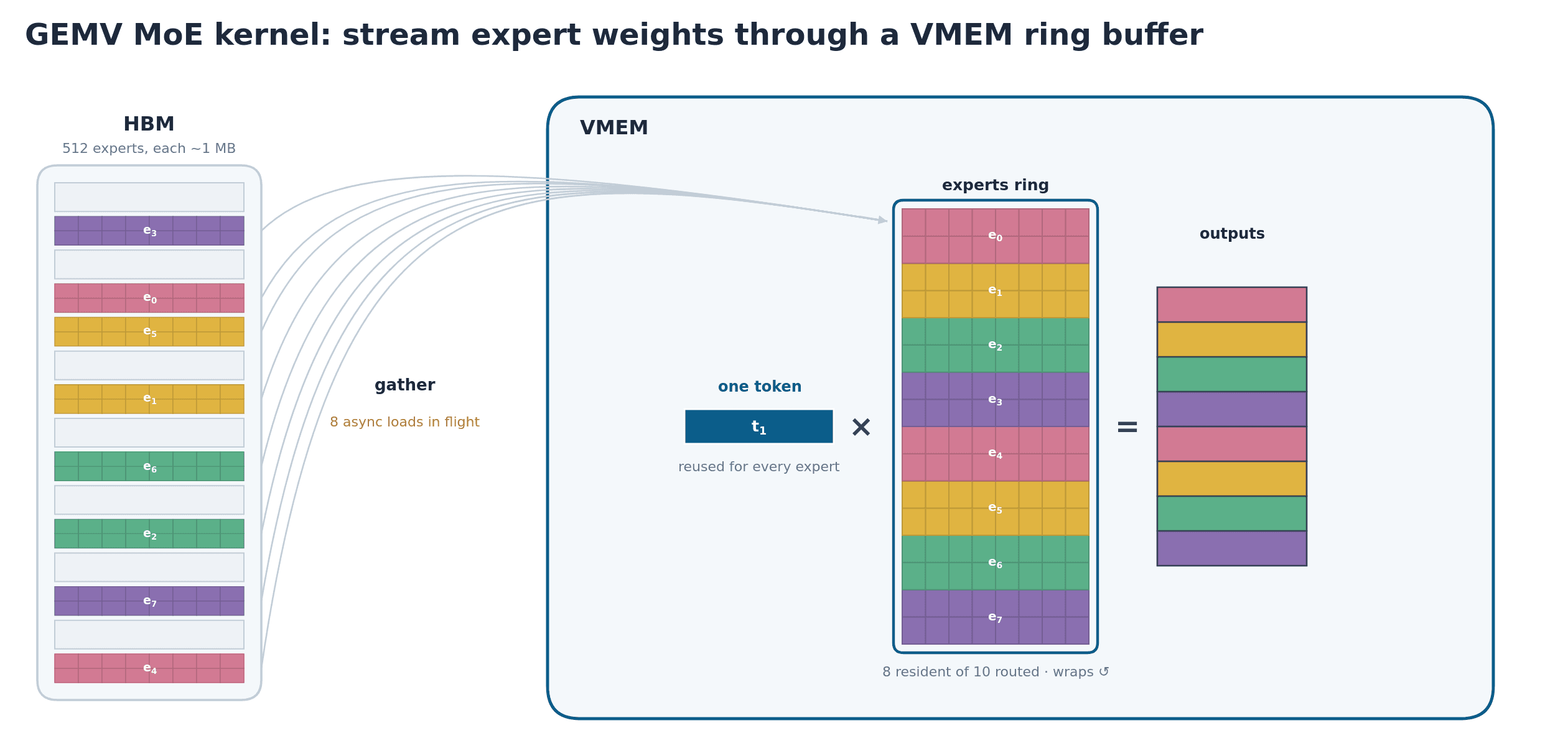
Since the expert calculation time isn't very significant, it's easy to fuse the shared expert into this kernel instead of calculating it in a separate step, for a further gain.

In fact, we have so much room in VMEM that we can fuse the entire gate+up+down MoE block with no global memory round trip! We found this fusion has mixed impact on performance depending on the exact concurrency, and should be conditionally enabled.

Making the CPU keep up

At some point, our device step got very close to the host step, and we were nowhere near our final goal. It was clear the performance targets would require an intervention on the host side as well.

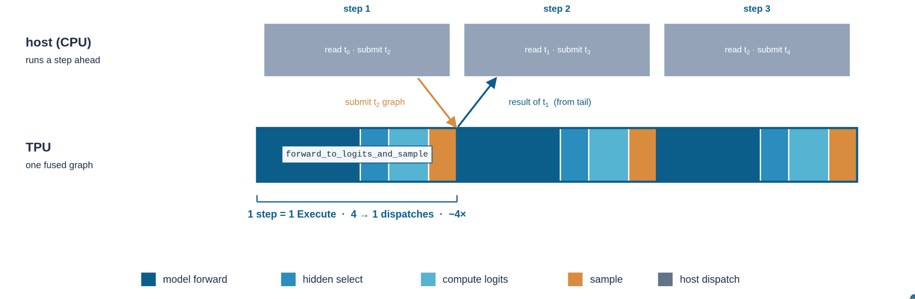
TPU inference relies on compiling, validating and submitting massive operation graphs. A model of Qwen's size has over 1.5k graph nodes that need validation. Originally, these were divided into four mid-sized subgraphs, corresponding to different tasks necessary to keep the model running, feed it input and receive its output. Fusing all these into a single graph reduced the host-side submission overhead nearly by half, unblocking further device-side gains. At the moment of implementation, this resulted in +16% tok/s/user. Notably, the fusion is fully compatible with vLLM async scheduling:

We covered only some highlights of our work — we also reworked the GatedDeltaNet kernels, customized vLLM scheduling, enabled different multi-node setups... but that's a story for another time. We are very excited about the unique capabilities of the TPU architecture. Prepare for more technical deep dives coming soon!

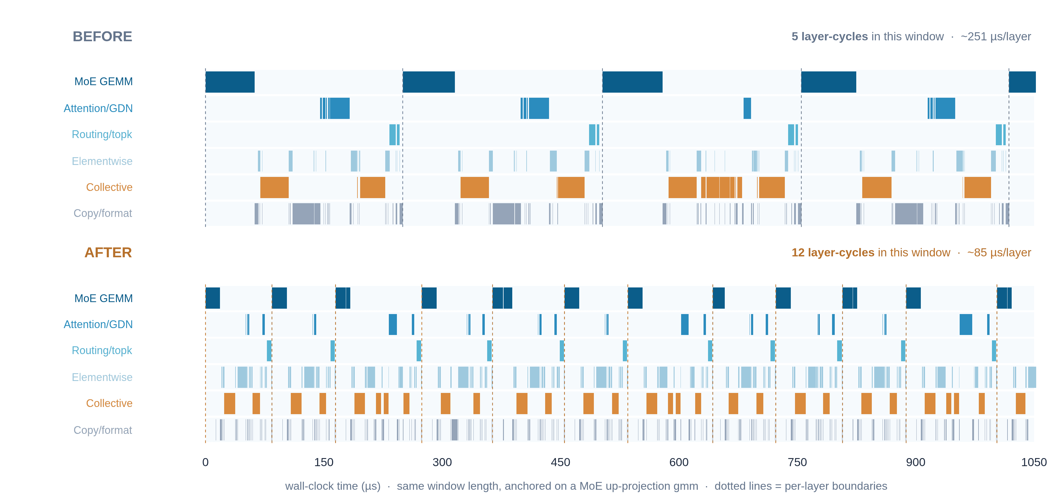
Real-world TPU profiling data of Qwen decode at a concurrency of 1. Makora's vLLM build calculates three layers by the time the stock build calculates one. The heterogeneous layers are visible in the chart (every fourth layer has full attention instead of GDN).

So how did we achieve these results? Below, we’ll walk you through the principles of our agentic workflows.

What does an agent see?

When trying to automate an expert's workflow, you need to understand what information is relevant for the expert's decisions and expose it to the coding agent. All the tooling should be designed much like it is for a human — it should minimize the possibility of using it wrong. An LLM can get distracted through context rot just as well as a tired human operator!

When optimizing an LLM for — in our case — a TPU cluster, your agents will need:

• a predictable environment, not dirty from previous experiments on a given machine, with an easy way to upload code changes and ensure no parallel agents are interfering

• scripts to capture high-level metrics such as TPOT, TTFT; there are right and wrong ways to benchmark, so for every important metric, the agent should have one canonical way of obtaining it

• CPU and TPU step time for decode and prefill — do you have a method that measures them correctly? Are you sure you're not miscounting one waiting for the other? What about multiple CPUs and multiple TPUs?

• a way to capture and review profiling trace data; TPU profiling traces are opaque Protobuffer binaries readable only by the XProf GUI; despite advances in LLM vision, your coding agent will have a terrible time trying to interface with a complex GUI

• a way to examine how your operations are lowered as close to hardware as possible, such as operation graphs (HLO on TPU), assembly or at least a compiler's intermediate language

• a way to map low-level primitives to your PyTorch or JAX code

All these problems are quite tricky, and even a Mythos-level model will struggle to get all of this correct every time. On the other hand, even a weak model is capable of impressive performance engineering feats if you provide a toolchain that fits the workflow. Makora’s custom toolchain allows coding agents to efficiently analyze, profile and optimize TPU workloads, unlocking powerful capabilities not reachable in standard coding harnesses.

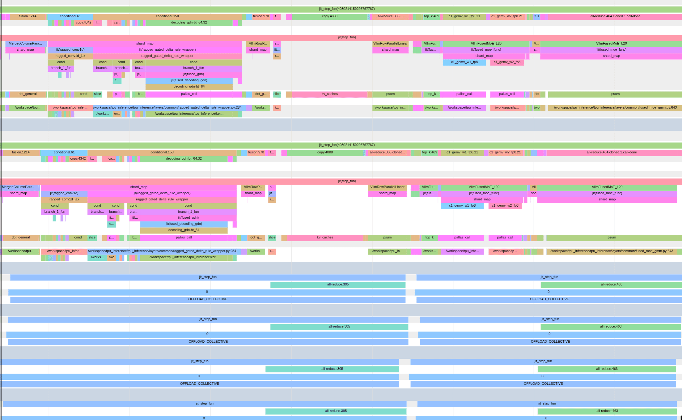
A single decode step in the XProf GUI — great for a human operator, difficult for an agent to understand.

Customizing the harness

In the course of this project the limitations of existing coding harnesses such as Pi, Claude Code and OpenAI Codex became apparent. Our toolset built to bridge these gaps later turned into Makora Swarm, an internal meta-harness that orchestrates multiple coding agents and faciliates agent-to-agent communication.

A fundamental element of our workflow is structured handoffs. The Claude model family is familiar with this concept out of the box, and when asked to provide a Markdown handoff note, will intelligently fill it with a streamlined description of the issue. In fact, we found asking an agent to handoff the current state to its next iteration works better than the builtin /compact command! This way we avoid context rot while accidental "side quest" discoveries made by agents can be properly resumed later. A deeply confused agent can handoff its investigation to a fresh instance and get its problem solved in five minutes, as opposed to wasting hours spinning in place with wrong assumptions.

For our purposes Claude subagents were nearly useless. Their communication bandwidth with the host agent is limited - they rely on one-shot instructions and can rarely acquire more context. On the caller side, context loss makes following up on their work impossible. Instead, Makora Swarm automatically spins up full handoff sessions, tracks tasks in a persistent queue and assigns TPU nodes to the agents that need them.

For tooling, we favor CLIs over MCPs. We make extensive use of skill .md files when our agents start repeating a workflow, and provide a short overview of each tool in CLAUDE.md.

The specific roles of each agent were dynamic and shaped by a human engineer's needs. Soon, common research, design, validation and integration phases emerged. In the middle of our sprint, Cloudflare published their Mythos workflow for security engineering, and we were surprised to discover we arrived at very similar methods in parallel.

Profiling data — if there is no CLI, it doesn't exist

Since the TPU ecosystem lacked a general purpose CLI for reading profiling traces, we built the internal jaxinspect tool to bridge that gap. This way, our coding agents could issue various queries against collected profiling data, such as:

• hotspot analysis with FLOPS / HBM / MXU utilization and Python source line attribution,

• temporal overlap between operations to understand situations like all-reduces hiding TPU kernel execution time,

• list of microsecond-level start/end/duration data of each instance of a specific op,

• a hierarchical vLLM module tree with aggregated device time, HBM and FLOPS contribution,

• a given op lowered into formatted HLO code, as executed on hardware

Soon, we found ourselves reaching for jaxinspect over XProf in our terminals, as loading and visualizing gigabyte-sized traces was overkill for many questions we wanted to ask. Armed with this tool, coding agents were able to investigate performance issues end-to-end and present trustworthy conclusions to their operators.

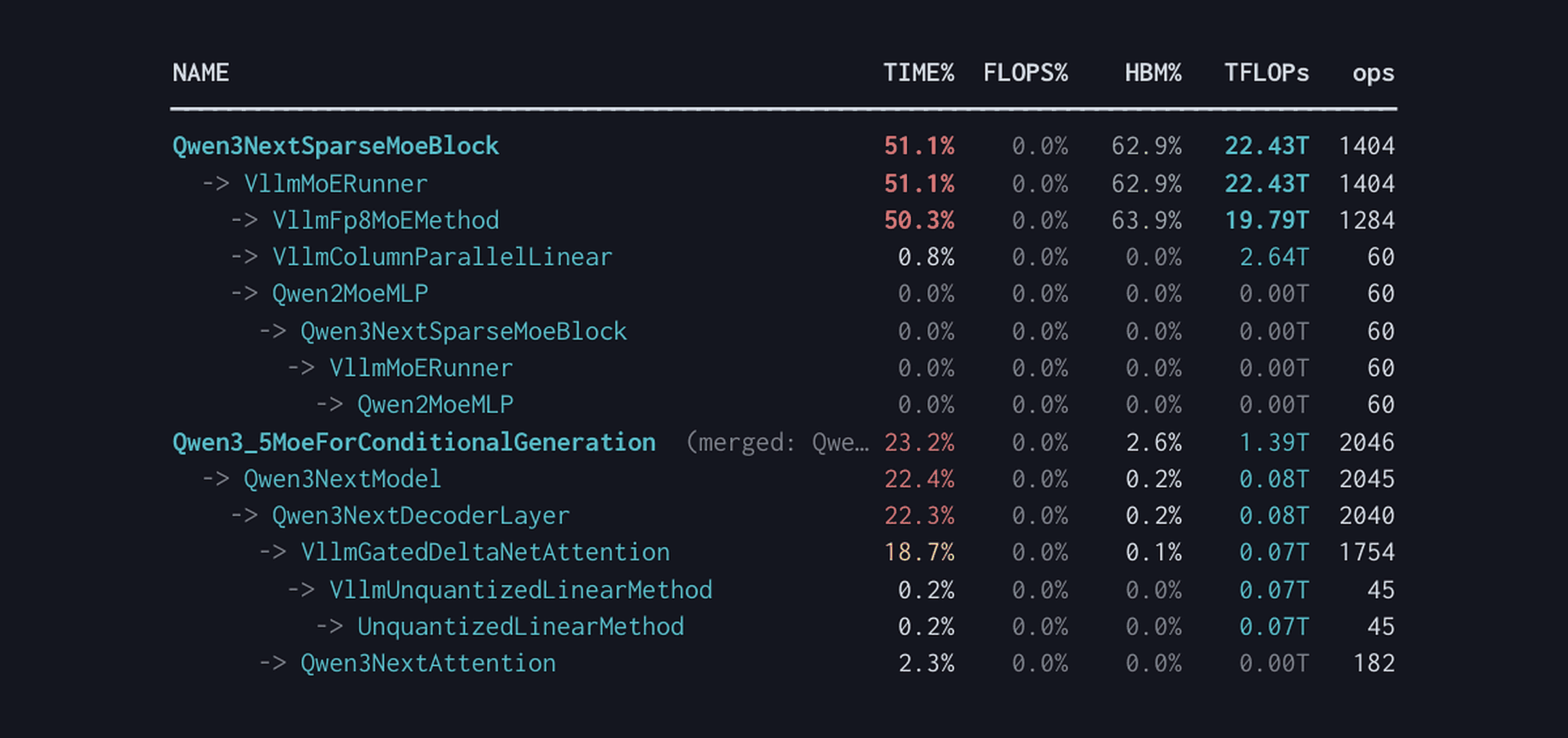
Example jaxinspect outputs.

0% FLOPS across the board is a profiling artifact — Pallas kernels on Ironwood do not collect this metric.

Teaching the agents how to benchmark

Early in the project we discovered coding agents can't write microbenchmarks at all.

While the JAX/XLA ecosystem is not as widespread in the training dataset as PyTorch/CUDA, we were still surprised to see LLMs routinely make basic mistakes:

• a time.perf_counter() loop that timed the host instead of the device,

• a jax.lax.fori_loop to amortize the dispatch cost; on the surface it looks solid, but it compiles the repeated calls into a single graph, allowing uncontrolled buffer reuse, invariant hoisting and other unexpected behavior,

• partially avoiding the fori_loop issue via in-loop dynamic_slice (indexing into one big buffer each iteration), adding gather/copy work that inflated kernel time and still linked the kernels into a dependency graph

To resolve these issues we had to provide a common microbenchmark template. The canonical methodology we settled on was:

1. Build N independent input sets — one per call, with no data dependency between calls

2. Issue the N JIT'd calls in a plain Python loop — not a JAX fori_loop inside a jax.profiler.trace

3. block_until_ready() once, at the very end

4. Recover the per-call on-device time spent from the resulting trace with jaxinspect.

import jax
import jax.numpy as jnp

@jax.jit
def kernel(*inputs):
    return my_pallas_kernel(*inputs)

inputs = [make_inputs(seed=i) for i in range(N)]

kernel(*inputs[0]).block_until_ready() # warmup

jax.profiler.start_trace(out_dir)
for x in inputs:                 # plain Python loop, not `fori_loop`!
    out = kernel(*x)
out.block_until_ready()
jax.profiler.stop_trace()

import jax
import jax.numpy as jnp

@jax.jit
def kernel(*inputs):
    return my_pallas_kernel(*inputs)

inputs = [make_inputs(seed=i) for i in range(N)]

kernel(*inputs[0]).block_until_ready() # warmup

jax.profiler.start_trace(out_dir)
for x in inputs:                 # plain Python loop, not `fori_loop`!
    out = kernel(*x)
out.block_until_ready()
jax.profiler.stop_trace()

import jax
import jax.numpy as jnp

@jax.jit
def kernel(*inputs):
    return my_pallas_kernel(*inputs)

inputs = [make_inputs(seed=i) for i in range(N)]

kernel(*inputs[0]).block_until_ready() # warmup

jax.profiler.start_trace(out_dir)
for x in inputs:                 # plain Python loop, not `fori_loop`!
    out = kernel(*x)
out.block_until_ready()
jax.profiler.stop_trace()

import jax
import jax.numpy as jnp

@jax.jit
def kernel(*inputs):
    return my_pallas_kernel(*inputs)

inputs = [make_inputs(seed=i) for i in range(N)]

kernel(*inputs[0]).block_until_ready() # warmup

jax.profiler.start_trace(out_dir)
for x in inputs:                 # plain Python loop, not `fori_loop`!
    out = kernel(*x)
out.block_until_ready()
jax.profiler.stop_trace()

So why do we need performance engineers, again?

All this automation might lead you to believe performance engineering is finished as a career, and a swarm of Claudes will now optimize everything for you. In our experience this is not the case.

The critical breakthroughs of the Qwen-3.5 sprint came from expert insight into how the model architecture, hardware architecture and profiling landscape mesh together. We made many discoveries through LLM-human dialogue, exploring possibilities, quickly running improvised PoCs and reviewing the LLM's suggestions through a critical lens.

The optimal performance engineering workflow remains an unsolved problem and will likely stay a moving target as model capabilities are pushed further. At Makora, we are determined to stay at the forefront of this technological revolution, making your models faster than you ever thought possible.